
Most business questions involve grouping and aggregating data. For example, we might want to examine sales by product category. Or else, we might be looking at profit margins by customer. Even when charting business performance over time, we are grouping our data by month or quarter. Therefore, you’ll find that .groupby() may be the method you use most often in pandas.
Grouping and aggregating data with .groupby()
Let’s use Question 4 of the Tableau exam prep guide as a case study for grouping and aggregating data. The question is: “What is the percent of total Sales for the “Home Office” customer segment in July of 2012?”
First, before we do any aggregating, we need to filter the data. After all, we’re only interested in sales for one month – July 2012. Since the order dates do not have times, we can filter the dates of interest using .between, starting on 1 Jul and ending on 31 Jul. Next, we will group the data by the column “product_category”, summing the “sales” in each category.
Most importantly, always remember to filter your data before grouping! For reference, you can use this post as a refresher on filtering if needed.
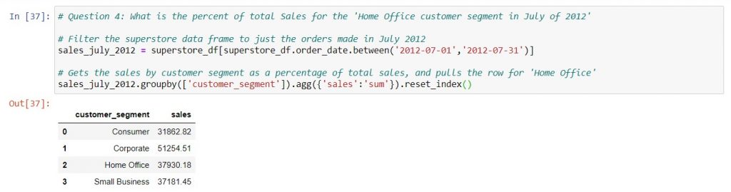
Syntax: pivot_table_name = dataframe_name.groupby([‘group_column‘]).agg({‘agg_column‘: ‘sum’})
You’ll see that in the round brackets after .agg, you are putting in a dictionary. This dictionary will map the data that you’re aggregating to the functions you want to use. Just like the aggregation functions in SQL (see here), you can choose from many common function types. Most often, you will use ‘sum’, then possibly ‘size’ (which is the same as “COUNT” in Excel or SQL), ‘mean’, ‘max’, ‘min’, and ‘std’.
Think about Excel pivot tables when using .groupby
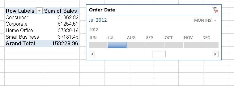
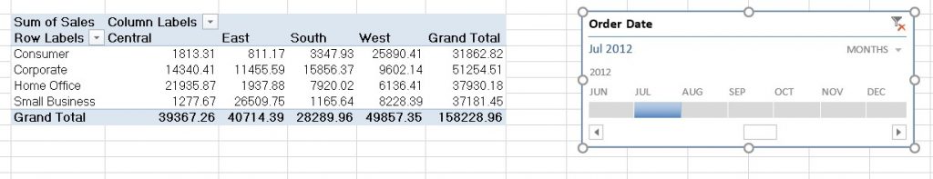
For the example above, we could have pulled the same numbers using Excel pivot tables:
- Insert a timeline on “Order Date” to select Jul 2012
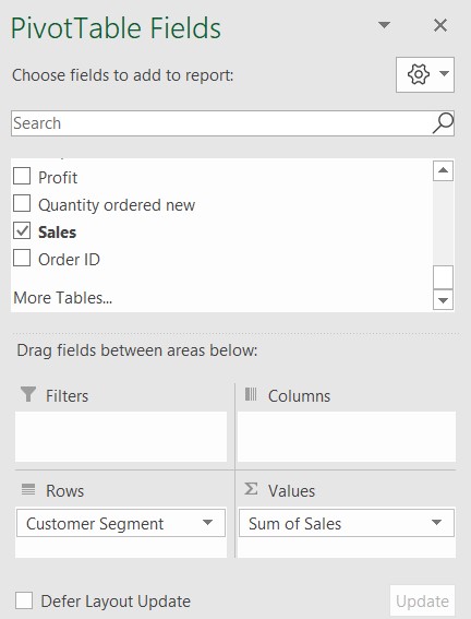
- Pull in “Customer Segment” to “Row Labels” and “Sales” to “Values”, setting the value field settings to “sum”
If you break down the .groupby method syntax into the equivalent processes of creating a pivot table, you might recall them more easily.
- First, in the round brackets right after .groupby, put a list of the column names you want in the “Rows” of the pivot table. Remember that a list uses square brackets, and that each column name is a string (within single quotation marks). Put them in the order that you want them in the pivot table (i.e. the columns from left to right).
- Second, in the round brackets after .agg, put a dictionary of the metrics that you want in “Values”, mapped to the aggregation functions that you want to use. Think of the aggregation functions as what you would select in “Value Settings” for each metric. You can aggregate a metric in more than one way, by putting a list of aggregation functions. Remember to write each function name as a string!
Putting it all together: a worked example
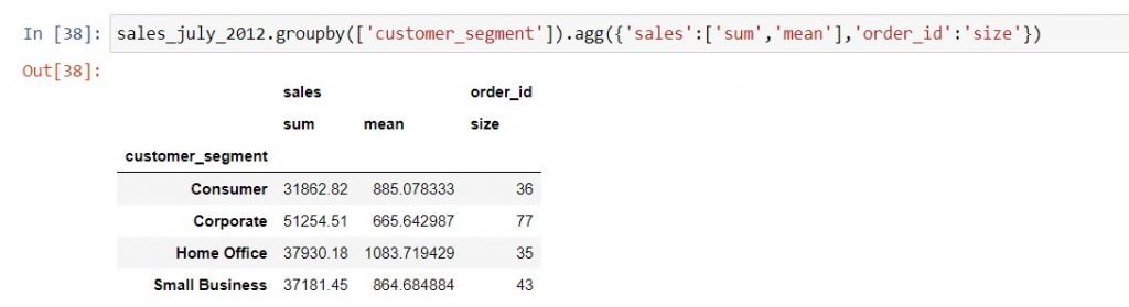
Let’s say we want to look at the total sales, average sales per order, and total number of orders in July 2012. How would this work in Excel and pandas?
In Excel, we would pull “Sales” in twice, selecting “Sum” in the first instance and “Average” in the second. Next, we would pull in “Order ID” to “Values”, and select “Count”. The result would look like this:
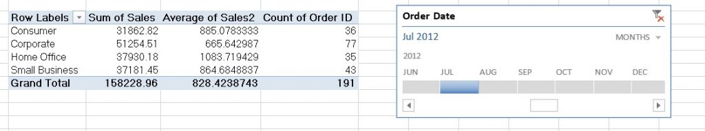
Using the instructions above, we can reproduce the same pivot table in pandas with .groupby as below:
Pivoting data with rows and columns
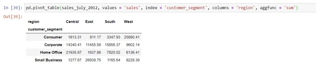
Now let’s say we want to look at the total sales grouped by customer segment and region. Using Excel, we can create this table by pulling “Region” into the “Columns” of the pivot table:
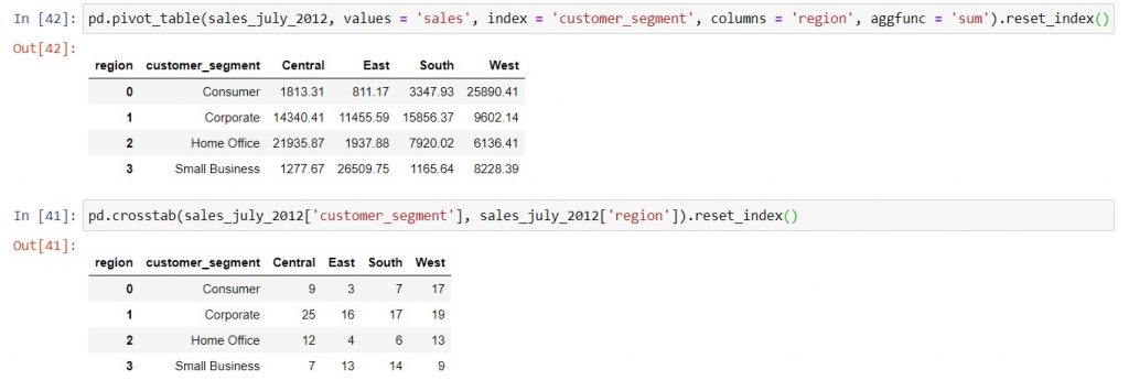
Syntax: pivot_table_name = pd.pivot_table( dataframe_name, values = ‘metric_column_name‘, index = ‘row_column_name‘, columns = ‘column_column_name‘, aggfunc = ‘sum‘)
Pandas also has a pivot_table function that replicates this type of structure. You can break down the syntax of the arguments in the following way:
- Firstly, name the DataFrame that this pivot table will get its data from. This is equivalent to selecting data from a worksheet in Excel to create a Pivot Table, and setting up the filters. Therefore, remember that the DataFrame must be filtered before calling pivot_table, same as for .groupby!
- Secondly, pick the category that you want to put into “Rows”, and name that column (as a string) in the “index” keyword argument. Remember that in DataFrames, the index denotes the rows!
- Thirdly, pick the category that you want to put into “Columns”, and name that column (as a string) in the “columns” keyword argument.
- Lastly, pick the metric that you want to aggregate by the row-column split, and put its column name (as a string) into the “values” keyword argument, as well as the “Value Settings” you would have given it in Excel under the “aggfunc” keyword argument. This works for all aggregations except counting, which we will discuss later.
The output of the pd.pivot_table function is a DataFrame, as shown below. You can either give it a name to save and write it to Excel, or see the numbers within the Jupyter notebook by running a cell with the code.
Counting the number of data rows across rows and columns
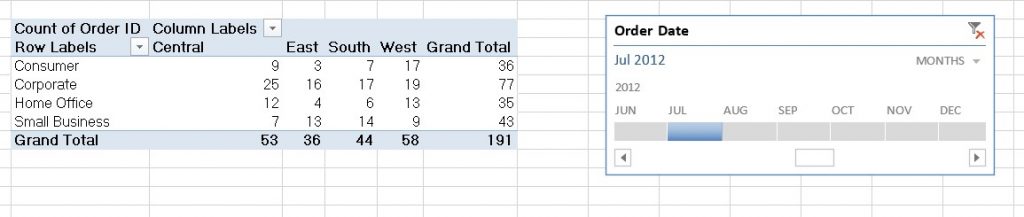
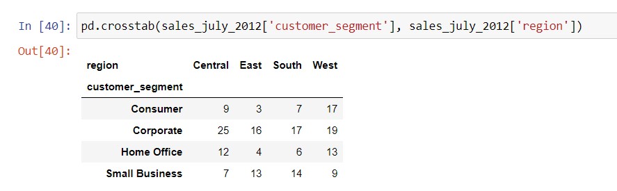
Earlier, we mentioned that pd.pivot_table will not work with “count” aggregation, such as if we wanted to count the order ID’s by customer segment and region. Instead, we need to use the pd.crosstab function to pivot the number of rows in the data set across two different categories.
Syntax: pivot_table_name = pd.crosstab( dataframe_name[‘row_column_name‘], dataframe_name[‘column_column_name‘])
Here’s a side-by-side comparison of how the pivot tables would look in Excel, vs. in pandas:
Be careful of what you want in the index of the pivoted DataFrame
The index of a DataFrame is a pandas Series containing values that identify different rows of data. As you may have noticed, any DataFrame that you create using .groupby, pd.pivot_table, or pd.crosstab will have the category values that you put into the pivot table’s rows as its index. You can bring these values into the columns of the DataFrame and replace the index with the usual row numbers by adding .reset_index() after calling any of these functions or methods.
In this post, we’ve covered:
| Things you would do in Excel | Equivalent task in Jupyter notebooks |
| Create a pivot table with categories in the rows and one or more metrics and aggregation functions. | Use the .groupby method, where you can group with multiple categorical columns, and also map multiple values to different aggregation functions using a dictionary. |
| Aggregate a single metric by two categories in rows & columns (i.e. creating a heatmap) | Use the pd.pivot_table function for all types of aggregation except counting. For counts, use the pd.crosstab function. |
Technical references
| Methods / functions | Pandas documentation |
| .groupby | There are a few different types of syntax you can use for .groupby. This post highlights the most versatile and easy to understand version, the full documentation is here in case you encounter other versions in your colleagues’ code. |
| pd.pivot_table | The function has a few other keyword arguments that might prove useful, documentation is here. |
| pd.crosstab | Similarly to pivot_table, has a few other keyword arguments that might be useful. Official documentation is here. |
| .loc and .iloc | If you are looking for a specific value inside a DataFrame, these are useful methods to know. The documentation is here for .loc which relies on row and column names to pull out a value, and here for .iloc which uses the numerical position of a row or column. Specifically, numerical positions are counted starting from zero from top to bottom for rows, and from left to right for columns. If you come across colleagues’ code in Python 2, .ix works similarly to .loc and .iloc. It is now deprecated, which means that you cannot use it when writing new code in Python 3. However, that shouldn’t be of concern as .loc and .iloc are easier to understand. |
| .to_flat_index | The official documentation is here but doesn’t show much. See below example on how to create easily readable columns when grouping on multiple metrics and aggregation functions. |
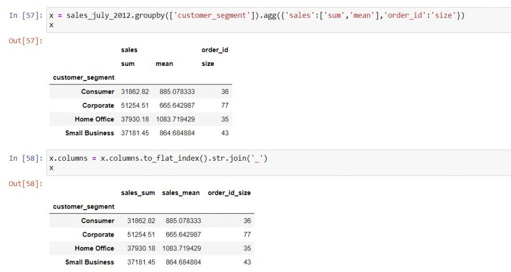
Flattening the column names when you group on multiple aggregation functions
When you group a metric using more than one aggregation function, your column names will be stacked in two rows. Subsequently, if you want to navigate the resulting DataFrame easily, you need to flatten the column names. To this end, you can use the .to_flat_index() method. For instance, you can do this:
Review on strings, lists and dictionaries
Lastly, the syntax examples and notes should provide some guidelines on how to set up strings, lists and dictionaries. However, if you need a refresher, you can go to Python For Everybody by Prof Charles Severance. Strings are here, lists are here, and dictionaries are here.