
Now that you’ve set up your Jupyter notebook, you can start getting data into it. To this purpose, this post discusses how to read and write files into and out of your Jupyter Notebooks. Furthermore, it tells you about the Python libraries you need for analyzing data.
First things first: Essential Python libraries
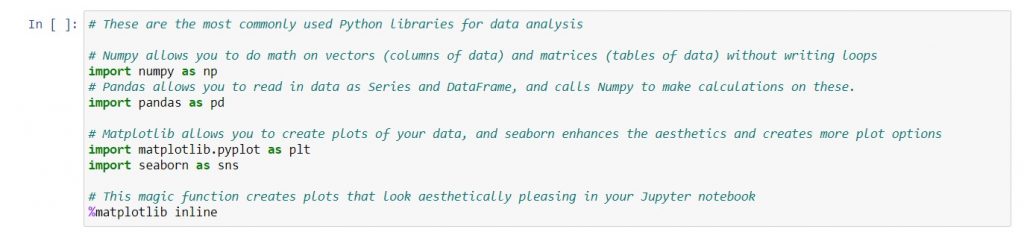
Your Jupyter notebook will contain cells, where you can type small pieces of code. Firstly, you’ll need to import the necessary Python libraries, before you can read or write any files. These are pre-written software packages that have specific purposes. For your needs, the two most important ones are numpy and pandas.
What are numpy and pandas?
Numpy is an open-source (free) Python library, which supports scientific computing. Because of numpy, you can make calculations on columns of data, without writing a program to loop through every value in that column. You can technically name numpy anything you want, but it’s standard to use “np” as above.
Pandas is also open-source, and stands for “Python Data Analysis Library”. As mentioned in the intro post to this series, it stores data as DataFrames and Series. These two structures enable you to navigate and manipulate your data. Again, “pd” is a standard short form to name pandas when you import it.
What are Python reserved words?
You might be wondering why the words “import” and “as” become green when you type them. This is the notebook’s way of telling you that these are Python reserved words. That means, Python uses these words for a specific purpose, so you cannot use them as names for any values that you create in order to manipulate (called variables). You can find a full list of Python reserved keywords here.
Why are there hash (#) signs in front of some of the text?
When you put a # (hash) sign in front of anything you type in your Python editor, it will become a comment. This is useful when you need to explain your code to someone else. With the # sign, Python knows to ignore that particular line when running your code.
Matplotlib and seaborn are second-priority for now. We’ll revisit them later.
Matplotlib and Seaborn allow you to create charts in Python. They’re extremely useful, but you’ll need to learn how to write the code. For simplicity, just understand for now that they exist, but we won’t prioritize them yet. If you can use pandas and numpy to simplify your data enough for creating a quick chart in Excel, you will already save a lot of time. This post explains why, but reader beware – it’s long!
Read and write files into Jupyter Notebooks
Now that you have imported pandas, you can use it to read data files into your Jupyter notebook. If you are reading data from a flat file, put it in the same folder as your Jupyter notebook, so that you won’t have to create complicated paths to the file. After Python reads the file, it will save the data as a DataFrame which you can then manipulate in your notebook. We will go through 4 common file formats for business data: CSV, SQL queries, Excel, and text.
1. Comma-separated (CSV) files
Most often, you’ll work with CSV files. That’s because if someone else pulled a large amount of data for you and saved it for later use in Excel, saving it as a .csv will take up much less space than as an Excel workbook (.xlsx). Also, when you first start practicing SQL, you may feel more comfortable downloading your output in .csv form, rather than reading directly from the query into your notebook. You’ll use the read_csv function in Pandas, such as the example below:

Syntax: dataframe_name = pd.read_csv(‘filename.csv’)
- In the above, grey words are placeholders for names you’ll need to customize. Red words are part of the format for calling the function.
- Putting pd. in front of the read_csv function tells Python to call the read_csv function from the pandas library. Because you imported pandas as “pd” earlier on, Python will know that “pd” refers to pandas every time you use it in your later code.
- The single quotation marks surrounding the file name tell Python to read this name as a string (i.e. text).
2. Getting SQL queries to output directly into your notebook
First, you need to write your SQL query as a string. This saves the query as a variable, which you can then refer to with the pd.read_sql function. As an example, this query came directly from the Survival SQL notebook:
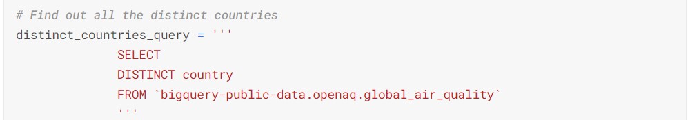
- Remember to put the query inside triple quotation marks! With the quotation marks, Python will read the entire query as a single string of text. Because queries often are easier to read if you split them over many lines, you need triple instead of single quotation marks.
- Consult your database engineers to get guidance on how to set up your database connection driver. They will show you how to set up a SQLAlchemy connectable, which you can declare as a variable named conn.
Then, you can get Python to directly read the output of your query by using this syntax:
dataframe_name = pd.read_sql(distinct_countries_query, conn)
In the above, I deliberately used the name of the sample query pictured, to show that you use the name of the variable you assigned the query to. Unlike the other examples where you refer to a filename as a string to search for in your folder, Python will take this variable and then read it. So, you should not enclose the query name in quotation marks when using pd.read_sql.
3. Excel workbooks (.xlsx or .xls)
You may need to read data from an Excel workbook if you’re working with files from an external vendor. If the file has clean columns of data, you can use the same syntax as the read_csv example above, just replacing pd.read_csv with pd.read_excel. But in case you have a messy file, here are some useful keyword arguments to know:

Syntax: dataframe_name = pd.read_excel(‘filename.xls‘, sheet_name = ‘Sheet1‘, skiprows =18, usecols = [2,3,4,5], header = na_values =[‘…‘])
- Colour-coding: grey denotes placeholders that you will customize. Essential syntax for calling the function are in red, and purple syntax are optional for the keyword arguments that you may need on a case-by-case basis.
Indicate where in the Excel file to read the data.
- sheet_name: If you have more than one sheet in the Excel file, this tells Python which sheet to read. You need to give the sheet name as a string (use single quotation marks).
- skiprows: If the data doesn’t start on the first row of the Excel sheet, you need to give skiprows an integer (i.e. a whole number without decimal points) to show Python the row where the data starts. For example, skiprows = 18 reads data from rows 19 onwards in the Excel sheet.
- usecols: When your data doesn’t start in the first column of the Excel sheet, you need to tell it which columns to use. Almost always you need many columns of data, so you need to specify them in a list. The square brackets are used to create a list in Python, and commas separate the individual items in that list. Because Python starts counting with 0 instead of 1, you need to adjust accordingly. For instance, usecols = [2,3,4,5] tells Python to read columns C, D, E and F in the Excel file.
Keyword arguments telling Python how to identify blanks
- na_values: Python thinks that missing data is always a blank cell in the Excel workbook. However, when people manually enter data, they may put ‘n/a’, ‘NA’, or ‘…’ like in our example above. Hence, you can give Python a string, or a list of strings (i.e. multiple strings in square brackets separated by commas) to tell it to put a blank in your data when it encounters that text. This will prevent your missing data from messing up future calculations.
Keyword arguments to identify or create column names
- header: Python assumes the first row contains the header (i.e. column names). If that isn’t the case, you can either use header = None, or give it an integer which tells it the row number to use. Because row numbers in Python start from 0, you have to subtract 1 from the row number in Excel. For example, header = 16 will tell Python to use the values in row 17 of the Excel sheet as the column names for the DataFrame.
- names: If you used header = None, you need to give your DataFrame customized column names. From our example above, the 4 columns of data are named “Country”, “Energy Supply”, “Energy Supply per Capita”, and “% Renewable”. When using this, remember to give a list of strings, and ensure that the number of column names equals the number of data columns. Name your columns from left to right, in the same way that you would in Excel.
4. Unformatted text files (.txt)
For reading .txt files, you will still use pd.read_csv, but with a different delimiter. Delimiters are the characters that split your data. For a .csv file, pd.read_csv uses a comma delimiter, by default. However, most .txt files use tab delimiters, so you will add on sep = ‘\t’ as another argument to indicate this. Therefore, your syntax would look like this:
dataframe_name = pd.read_csv(‘filename.txt’, sep = ‘\t’)
Writing a DataFrame to a .csv file
After you’ve worked on your data with pandas, you might want to export some of your output to a .csv file. Especially, you might be interested in doing this if you want to create charts in Excel. So, you would use this syntax:
output_dataframe_name.to_csv(‘data.csv‘, index = False)
- Unlike the earlier examples of reading data, .to_csv is a method, not a function. Don’t worry too much about the theory at this point, just note that in this example, you are not creating any new variables. Instead, you are applying the method .to_csv to a DataFrame called output_dataframe_name (a placeholder, you can call it anything you want when you create it in your code), which will trigger the action of writing the file.
- The above code will create a file called data.csv within the same folder as the Python notebook.
- index = False is a keyword argument to tell Python to exclude the index of the DataFrame when writing it. This will mean that your first column of data is also the first column you see when opening your .csv file in Excel. Otherwise, your first column would be the index column of the DataFrame. If you haven’t done anything to customize the index, usually the index column is like a row number reference for the DataFrame, starting from 0. We will discuss indices in greater depth later on in this series.
In this post, we’ve covered:
| Tasks you would do in Excel | Equivalent operation with Jupyter notebooks |
| Import the numpy and pandas libraries because you need them for data analysis. | |
| Populate your data sources by putting them in sheets | Read data from different sources into DataFrames using pd.read_csv, pd.read_sql, or pd.read_excel. Think of each DataFrame as the equivalent of an Excel sheet. |
| Write a DataFrame to a .csv file, using .to_csv. This allows you to further work with the data in Excel, e.g. to create charts. |
Technical References
After you feel ready for all the technical details, you can use these resources to dive deeper:
Python concepts covered in this post
| Concepts | Chapters in Python For Everybody |
| Python reserved words Declaring variables | Chapter 2 |
| Strings | Chapter 6 |
| Lists | Chapter 8 |
| Functions | Chapter 4 |
| Object-oriented programming (methods) | Chapter 14 |
Official Pandas documentation for all functions and methods from this post
| Getting data from a .csv or .txt file | read_csv |
| Reading a SQL query | read_sql |
| Pulling data from an Excel file | read_excel |
| Writing data to a .csv file | .to_csv |