Your Jupyter notebook has read the data from your files and / or SQL queries. Therefore, you now have a DataFrame each for what would have been your data sheets in Excel. At this point, it’s time to inspect and explore your data.
Inspect what the first few rows of data look like
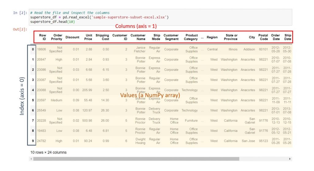
Firstly, to see the first few rows of your data, you can use .head(), as shown below. Within the brackets, enter the number of rows you’d like to see. And if you do not put any number inside, i.e. just type dataframename.head(), you’ll automatically get the first 5 rows in your DataFrame.
Syntax: dataframe_name.head(10)
Attributes of a DataFrame
Secondly, you can dive into different parts of your DataFrame. As mentioned in the intro post, a DataFrame is a class of objects. In non-technical terms, this means that it’s a type of data structure with specific characteristics. Also, it stores information on these characteristics into structures called “attributes”, so that you can see and manipulate them. Below are a few key attributes that may interest you:
- Columns: These are the names of the columns, analogous to the header row in your Excel spreadsheet. When you see axis = 1 in a colleague’s code, the code evaluates across the columns of the DataFrame.
- Index: By default, this is like the row numbers in an Excel spreadsheet, except that Python starts with 0 instead of 1. When you first read your data, it might not be sorted the way you want, so you might end up resetting your index after sorting. We’ll cover more of that in a later post. Furthermore, as you become more familiar with programming, you might set different columns within your DataFrame as the index to make it easier to search your data. When you see axis = 0 in a colleague’s code, the code evaluates down the rows of the DataFrame.
- Values: The values are a Numpy array, which basically means a 2-dimensional matrix containing all the data in your table.
- Shape: The number of rows and columns in your DataFrame (see below).
Explore your data using DataFrame attributes
You’ll probably be curious about the amount of data that you have. To achieve this, you can print the DataFrame’s shape, which will give you the number of rows and columns in your DataFrame. For instance, the DataFrame named superstore_df that I read into the notebook earlier has 9426 rows and 24 columns.
Syntax: dataframe_name.shape

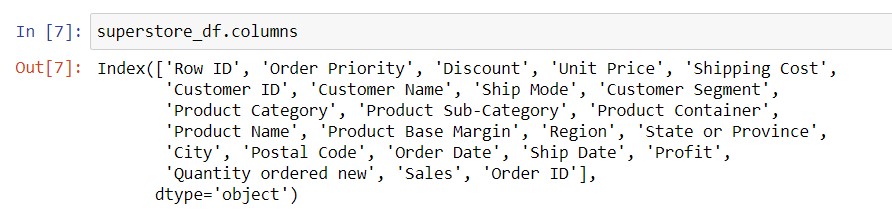
If your data has too many columns, .head() won’t give you all the column names because it wants to fit the entire DataFrame into your browser page. However, you can print the full list of columns using .columns. Similar to how we did it for .shape, you type dataframename.columns into a cell, then run it.
Syntax: dataframe_name.columns
Find out what is in a particular data column
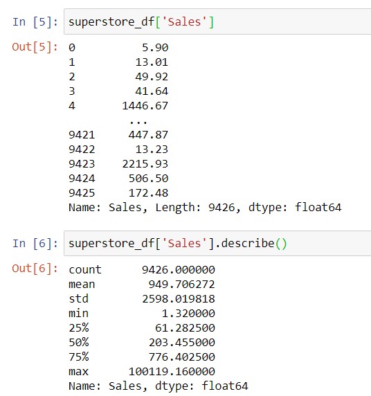
Some of your data will be numerical, which means that it’s expressed in numbers can be used in calculations. For example, the “Sales” column, which contains the dollar value of a particular order, is numerical data. Conversely, other data columns will be categorical, which means that it’s used for grouping your data. For instance, “Customer Segment” is categorical, as is “Region”, “City”, etc.
Before you start working with your data set, you may want to inspect the specific columns of interest, and sense-check what you see there. For numerical data, you’re probably interested in what representative values may look like, and also in the maximum, minimum and average values. Here is an example to help you get this information:
Syntax to get a column: dataframe_name[‘column_name‘]
Syntax to get key statistics in a numerical column: dataframe_name[‘column_name‘].describe()
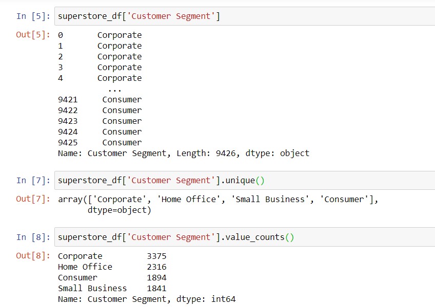
For categorical data, you might be interested in the different category names. Additionally, you may want to know how prevalent each category is in your data.
Syntax to get all the unique values in a column (usually categorical): dataframe_name[‘column_name‘].unique()
Syntax to get the number of rows in your data corresponding to each unique value in a column: dataframe_name[‘column_name‘].value_counts()
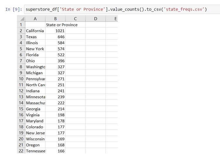
All of the above sense-checks will help you confirm that your data was pulled properly, before starting to do anything with it. Sometimes, the result of .value_counts() might be too big to display fully within your notebook, so you can use .to_csv (see this post) to write the output to a CSV file. If you use to_csv, your notebook won’t print the result inline. But when you open the .csv file, you will find the data, sorted with the value with the most rows first:
In this post, we’ve covered:
| Things you would do in Excel | Equivalent operation with Jupyter notebooks |
| Eyeball your data sheet by scrolling around and visually inspecting the data. | Print the first few rows of your data inline with head.(). Find the Get a full list of the column names with .columns. Slice the DataFrame to see data in a particular column. |
| Hover over a column of numerical data to get the number of values, sum and average. | Use .describe() to get summary statistics for a column. You get all the values that Excel gives you, plus also the standard deviation and quartiles. |
| Filter a column of categorical data to see the unique values. | Print out the unique values within your notebook, using .unique(). |
| Pivot a column of categorical data to find the most frequently occurring values. | With .value_counts(), you can get the number of rows with each category, with the most frequent categories first. |
Technical References
After a little practice, you might feel ready to dig into the theory behind each of these data structures. You might also remember the syntax and punctuation better if you understand the theory behind them – that is another good reason to refer to the Python For Everybody resources.
| Data you encountered in this post | Type of Data Structure | Resource |
| DataFrames you obtain by reading files or SQL queries into your notebook | DataFrame | Pandas documentation: DataFrame |
| Column of a DataFrame Output of value_counts() | Series | Pandas documentation: Series |
| Shape of a DataFrame (i.e. output of .shape) | Tuple | Python For Everybody Chapter 10 |
| Questions about syntax from this post | Conceptual overview | Where to dig deeper |
| Why do we use a period between the data frame name and .index, .columns, .shape and .values, but no round brackets? | These are attributes of your DataFrame. | Python For Everybody Chapter 14, Python Objects See a full list of the attributes of pandas DataFrames here. |
| Why are there round brackets for .head(), .describe(), .unique(), and .value_counts()? | These are methods that can be used on a Series or a DataFrame. | Python For Everybody Chapter 14 will also explain methods. Scroll to the bottom of this page to get all the methods applicable to DataFrames, and this page likewise for Series. |
| Why are there square brackets and quotation marks when you reference a column from a DataFrame? | You are slicing the DataFrame, hence the square brackets. The quotation marks express the column name as a string, and Pandas will turn that column name into a column index in its back-end to create the slice. | Python for Everybody explains list slicing in Chapter 8. Technically, Pandas is slicing a 2-dimensional array here, but the concept is similar. |