
Lately, I’ve been working through Think Stats by Professor Allen Downey. This book provides a novel way to learn statistics. Instead of formulas and theory, it teaches the same concepts with hands-on coding exercises. Because I am a business analyst, I identify with the practical approach of Think Stats. And today, I’d like to share my solution to the Think Stats “runner” problem in Chapter 3.
Outline of the runner problem
In this question, we’re in a long-distance race, and runners of different speeds are spread out throughout the entire course. Yet, a runner at the average speed might not see people running at his pace because he is less likely to pass them during the race. Read the question directly in the textbook here.
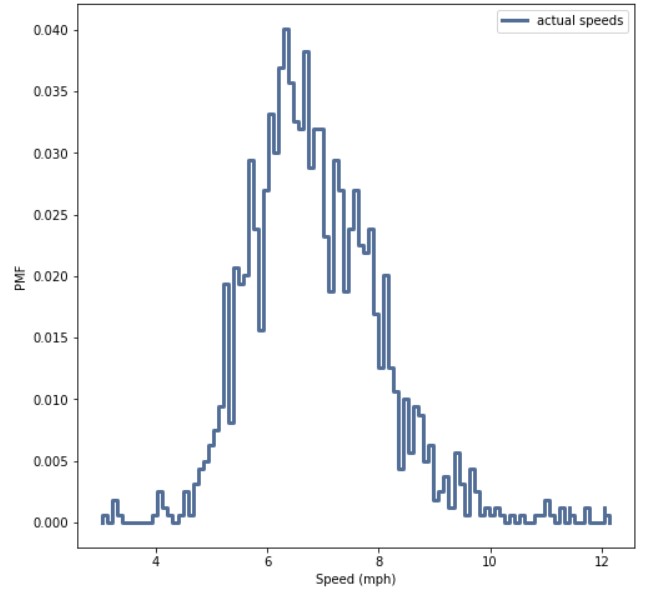
Prof. Downey gives us the actual runner speed distribution, as a probability mass function (PMF), and it’s a bell curve clustered between 6-8 mph. In this exercise, we follow a runner at 7 mph. Such a runner is at the mode of this distribution, so in reality, runners of his speed are the most common in the pack. But what does he perceive the speeds of the runners around him to be?
Step 1: Runners at the same speed
Prof. Downey tells us that the race has a staggered start, and spans 209 miles. So, I made these assumptions:
- Runners are equally likely to be at any mile marker on the course.
- The speed distribution of runners at any marker is the same and follows the bell curve above.
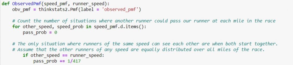
- Our runner is only concerned about runners who are on the course at the same time as him at some point. This results in 208 + 208 + 1 = 417 combinations of distance for every runner speed.
Since our runner will only see another runner at exactly his speed if they start at the same time, his probability of observing another runner at 7 mph is 1/417. Hence, this translates into the following code:
Step 2: Runners slower than our runner
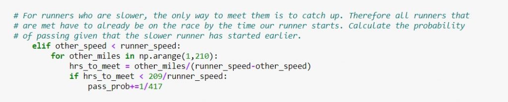
For our runner to meet a slower runner, the other runner has to already be in the race, and our runner will catch up with him before the finish line. Therefore, we can calculate the time (in hours) required for our runner to catch up with a slower runner for every possible distance gap. Each of the instances where the catch-up time is less than the time our runner takes to finish the race adds 1/417 to the probability, because we have 417 different possible distance gaps:
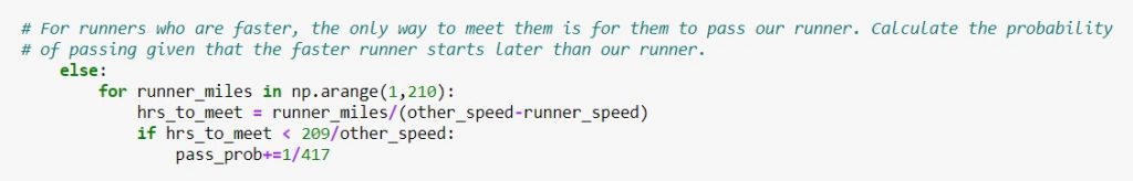
Step 3: Runners faster than our runner
Similarly, the only way our runner can meet a faster runner is when the faster runner starts later, then passes him. So, the same logic applies but with the roles reversed:
Putting it all together
Now, we know the probabilities of our runner meeting another runner, given the speed of the other runner. With Bayes’ Theorem, the probability of another runner being at that speed and our runner meeting that runner is the product of the two values:

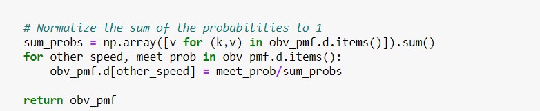
Lastly, a probability mass function represents relative likelihoods of the different outcomes, that add up to 1. So, we have to normalize all the values:
How did my solution compare with Prof Downey’s?
My approach was slightly more fanciful than Prof Downey’s proposed solution, because of my additional assumptions. Still, both approaches produced similar observed PMF’s. Our runners meet more other runners in speeds slightly faster or slightly slower than them, and few at their own speed. Therefore, they think the speed distribution is bimodal, and don’t realize that they are at the mode of the actual distribution.
The two differences in the solutions are:
- Prof Downey’s solution gives a higher probability to meeting a faster runner than mine
- It also gives a lower probability to meeting a slower runner than mine.
His solution is symmetrical as it divides each probability in the underlying PMF by the difference in speeds. Conversely, mine is slightly asymmetrical. It dives into the time taken to pass a given runner at a given distance gap with given speeds. Therefore, it’s more sensitive to small asymmetries in the speed / probability combinations on either side of 7 mph.

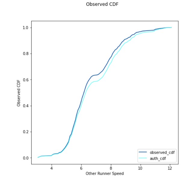
The cumulative distribution function (CDF) graphs of the two solutions also reflect this difference in bias. Note: While a PMF represents the probability of finding a runner at any one speed, a CDF represents the proability of finding a runner at less than or equal to a particular speed. Both solutions find our runner more likely to meet a slower runner than a faster one, but mine is more weighted towards slower runners than his.
Another twist: this is a relay race!
Actually, we aren’t following just one runner in this scenario. 209 miles is a long way for any one person to keep going at 7 mph! So, this situation only holds when we are following a team of 7 mph runners handing off to each other throughout the entire 209 miles. In reality, any one person probably runs 10-20 miles at most (a half or a full marathon). Therefore, I re-ran the calculation assuming that each runner covers 21 miles. In other words, the gap between our runner and other runners would be up to 20 miles ahead or behind (20 + 20 combinations), as well as the runners starting at the same time (1). This means substituting all probabilities to 1/41 (i.e. 20 + 20 + 1) and the race distance as 21. The resulting PMF looks like this:
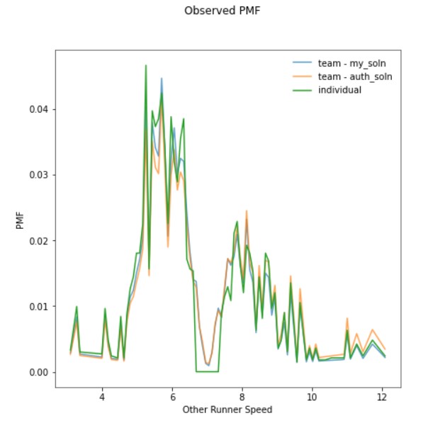
The dip in the probability of our runner encountering other runners close to his speed is even more pronounced, because the shorter distance gives him less opportunities to catch or be caught by them.
Hope you had fun reading this!